

In statistics, there are a multitude of paradoxes; These strange situations that challenge our intuition. Simpson’s paradox is probably the best known, often encountered and certainly one of the most intriguing. Described in 1903 by Yule, Simpson’s paradox also called Yule-Simpson effect, was then supported by Simpson in 1951. It is distinguished by a certain tendency for the set of combined data (all groups combined), but when we stratify or control by a group variable, the trend either reverse or cancel, so that it is impossible to deduce true from false.
A visual is better than words. Here is a hypothetical example (for a real example see below). Pictures below illustrate Simpson’s paradox for continuous data representing light colour (CCT, in Kelvin) and light intensity (illuminance, in lux). The graph on the left clearly shows a positive correlation: the more light intensity increases, the more the colour of the light becomes white.
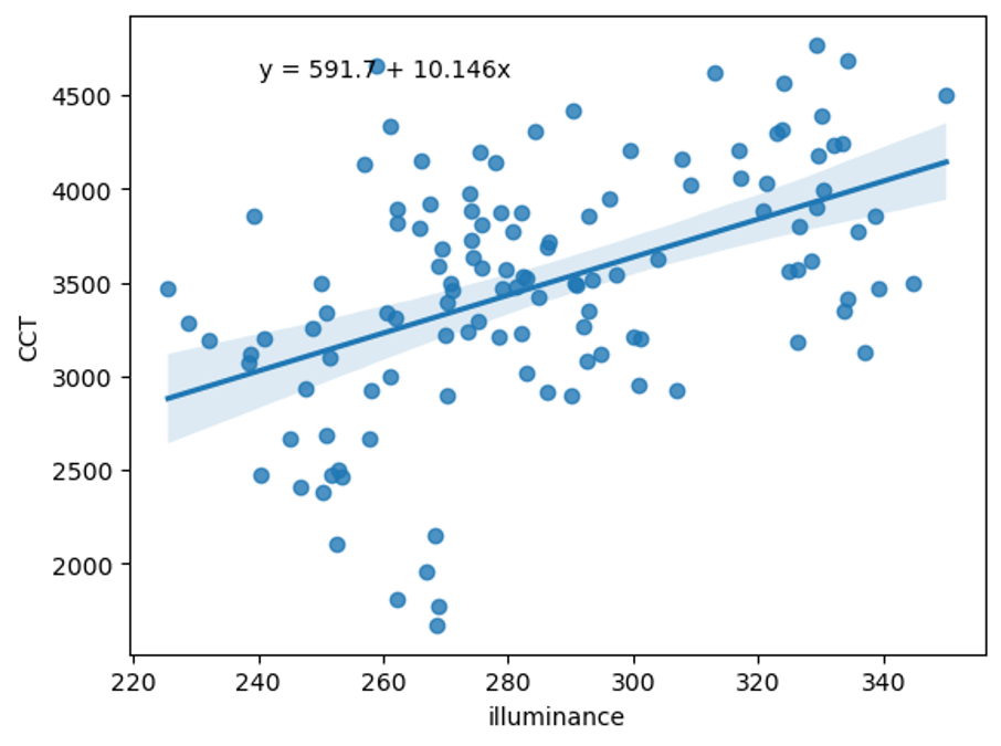
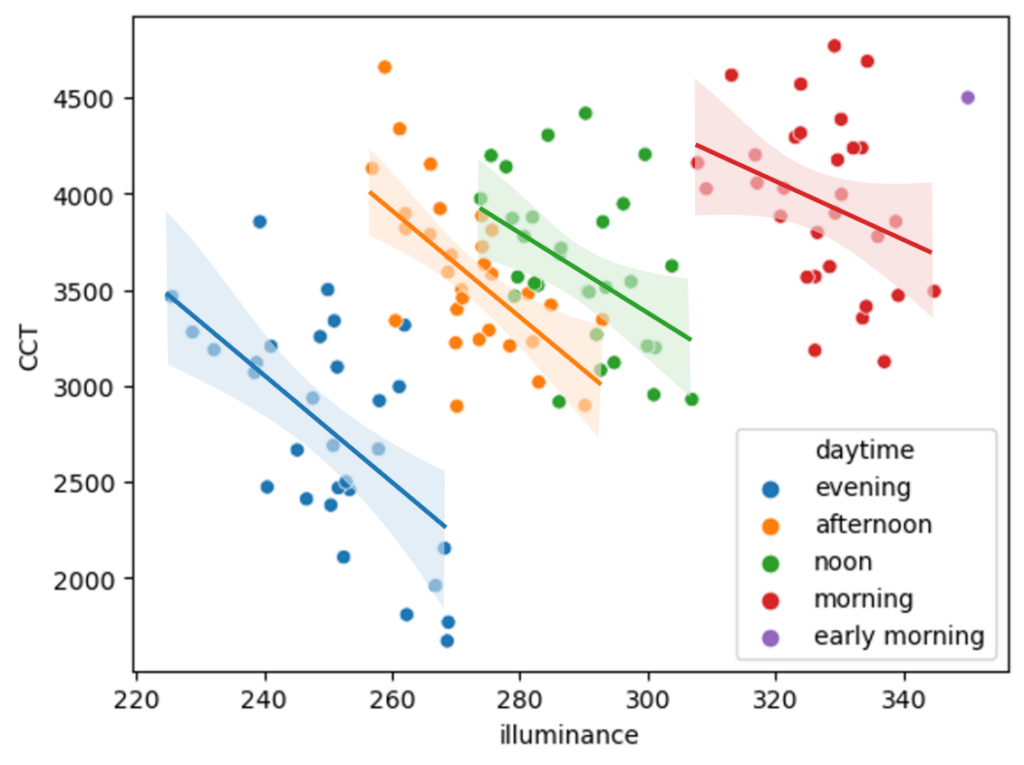
However when stratified by the group ‘daytime’ (early in the morning, in the morning, at noon, afternoon and evening), we see that it is the different groups that increase the CCT and the illuminance: the more we advance in the day, the more the CCT and illuminance are low.
We could therefore explain this paradox by the following diagram:
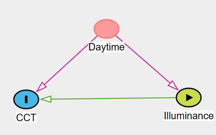
To solve this paradox, it will be necessary, as indicated by Dagitty, to condition by Daytime (see below, the next example for a detailed explanation of Simpson’s paradox resolution).
real example
The next example, was discovered when I was working in the field of old age pensions at the Federal Statistical Office. It is observable in the New Annuity Statistics (NRS) data on the amount of pension funds from Swiss pension funds, by type of combination and gender (this table for the years 2020 to 2024). It will probably also be observable in future years.
The same explanation is valid for all years. So here we will only take the example for the year 2024. The data concerned are reproduced below:
| Annuity only | Annuity and lump sum | |
| Men | 2,650 | 2,556 |
| Women | 1,571 | 1,484 |
| Total | 2,141 | 2,227 |
As indicated in bold, the amounts are higher for the combination ‘love only’ in women and men, on the other hand for the overall data, it is the annuity combined with the lump sum which shows the largest amount.
As soon as I was informed of the presence of this paradox in our data, I immediately thought of Judea Pearl and her scientific paper on Simpson’s paradox resolution: http://dx.doi.org/10.2139/ssrn.2343788. So I was quick to solve our paradox. Before presenting my approach, you have to take a slight detour through the maths that translate that the overall effect goes in one direction and the effect by controlling for a variable in the other. Here they are:
- Y will be the amount of the pension
- X will be the annuity combination, either annuity alone or combination annuity and lump sum
- Z will be sex, either men or women
The average of the amounts that differ for each group translates to:
The inversion of the total effect is as follows:
by the law of total expectation we get:
This means that to assess the amount difference between annuity only and the annuity and lump sum combination, it is necessary to make a weighted average of the averages of each sex. We therefore deduce that the weights:
are not the same for each pension combination.
So I got down to checking the proportions of choice of people according to sex.
| Annuity only | Annuity and lump sum | Total | |
| Men | 13,833 | 9,574 | 23,407 |
| Women | 13,224 | 4,449 | 17,673 |
| Total | 27,057 | 14,023 | 41,080 |
| Annuity only | Annuity and lump sum | |
| Men | 51% | 68% |
| Women | 49% | 32% |
| Total | 100% | 100% |
We therefore note that the two sexes take are well distributed in the annuity alone, but in the combination of rent and lump sum, there are more men than women. the fact that there are more men in the combination of rent and lump sum can pull the average up, so it will be necessary to stratified by sex, because it concerns two very distinct populations which influence the amount and the chosen combination.
From a causal perspective, several patterns can explain this paradox: a confusing variable, a mediator…, as described in Pearl’s paper.
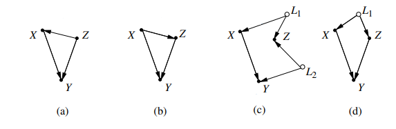
Of course, depending on the configuration, the intervention to obtain the resolution will be different. It will be necessary to condition/stratify by Z in diagrams A, B and D, but not in case C. In our case, similar to the hypothetical example, we probably find ourselves in the case A; The confounding variable:
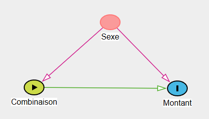
The right answer to solve this paradox of Simpson is therefore to stratify by sex. We can therefore conclude that taking an annuity only allows to get a higher amount in retirement than take a combination of annuity and lump sum. This answer is satisfactory and makes sense of a theoretical point of view.
P.S.: Unless, of course, this model is too simple and the reality much more complex, filled with unmeasured variables, such as the level of wealth, history of working life etc. 🙂